Principle of Virtual Transition
The Principle of Virtual Transition is used in Permanent Way alignment design to establish when a transition curve in not needed and design a sudden change in curvature.
The principle is defined in sheet B.3.4 of the Track Design Handbook – NR/L2/TRK/2049 (2010):
“The determination of maximum permissible speeds on curves without transitions involves the concept of a virtual transition.
Consider a coaching vehicle, having bogie centres C1 and C2, B metres apart, travelling at a uniform speed V km/h, from the straight on to a circular curve of radius R which is tangential to the straight at TP (see Figure 1). 
Figure 1. The principle of Virtual Transition
The vehicle moves with a uniform velocity in a straight line until the bogie centre C1 reaches TP. Here the motion of the vehicle begins to change as it passes on to the curve, and the vehicle gradually acquires angular velocity. The change continues until the bogie centre C2 reaches TP, after which the vehicle moves round the curve with uniform angular velocity.
The change of motion of the vehicle from straight to curve conditions takes place in a distance of B metres. The length B may therefore be considered as a virtual transition.
The value of B to be used is 12.2 metres which is the shortest distance between bogie centres of the British Railway coaches. Shorter wheelbase vehicles will suffer higher values of cant deficiency at switch toes and higher rates of change of deficiency elsewhere so the actual wheelbase of shorter (less than 12.2m bogie centres) passenger rolling stock should be used in speed calculations.
The value of 12.2m should not however be relaxed for vehicles with a longer wheelbase as the lateral thrust on track components becomes excessive.
Deficiency of cant is considered as being gained in the length of the virtual transition, commencing on the straight 6.1m before TP, and terminating on the curve 6.1m beyond TP.”
A similar definition can be found also in the informative Annex E of the European Norm for track alignment design BS EN 13803-2 (2006):
“This principle is based upon the assumption that a characteristic vehicle travelling over an abrupt change in curvature gains, or loses, cant deficiency (and/or cant excess) over a length equal to the distance between the bogie centres of the characteristic vehicle (B). This distance is also denoted virtual transition and is assumed to extend a distance B/2 each side of the abrupt change in curvature.”
The curvature variation over Virtual Transition
Although the Track Design Handbook, TRK2049, suggest that the principle could be also used over a variable cant zone, it is used only in areas where the cant is constant. In this case the presumed variation of the Cant Deficiency will be caused only by the curvature variation perceived at vehicle level, when passing over a point of sudden change in curvature. The angular velocity mentioned in the principle definition, is not explicitly considered a design constraint by the standard and none of the cant and alignment parameters, as they are defined today, are dependant of it.
Even though the standard does not specify how the cant deficiency varies over the Virtual Transition, in the alignment design this variation is considered linear, as for a real linear transition, the clothoid for example.
A more detailed graphical description of the principle is given in figure 2. When the reference vehicle (Figure 2.A) is passing over the straight with both its bogies, the point M (the centroid of the vehicle) is staying on the straight track centreline. As the first bogie, C1, is passing over the tangent point TP to the circular curve, the middle point M of the vehicle is describing a smooth curve of unknown curvature. After the last bogie, C2, is passing the tangent point and both bogies are running on the circular curve, the point M describes an offset of this centreline circular curve (see Figure 2.B).
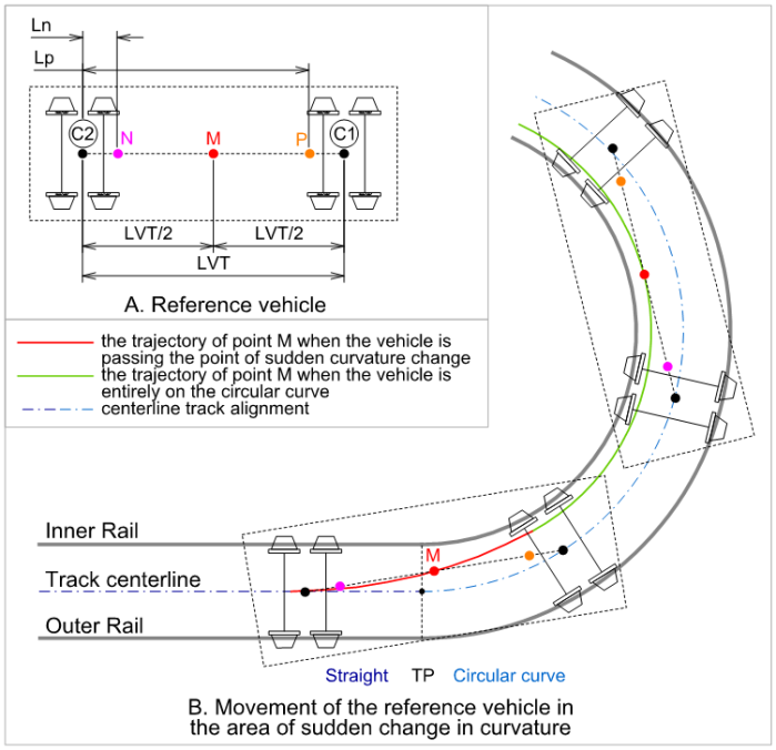
Figure 2. The trajectory of the middle point of the reference vehicle when passing a sudden change in curvature (not to scale)
There are different ways to find out how the curvature varies at vehicle level over the virtual transition, either using acceptable approximate methods as the ones from the Hallade realignment theory (Radu – 2003), precise using spline polynomial equations, or even graphical methods, measuring the versines of the curve drawn by M as the vehicle is passing the tangent point.

Figure 3. Finding the curve described by M (not to scale)
When the vehicle is passing the tangent point TP (see figure 3), the point C1 describes the centerline circular arc with the following equation:
 Using Taylor expansion for the square root, YC1 becomes:
Taking in to account the big difference between X and R, the boxed part of this formula is practically null. Hence, with acceptable precision, (2) becomes:

For X significantly smaller than R, as it is the case for a railway track curve, this demonstrates the equivalence between the parabola, defined by (3), and a circle, defined by (1), with a radius R equal to the distance between the focus point and the directix line of the parabola. This equivalence is known in analytical geometry as the osculating circle or the kissing circle of a parabola – circulus osculans.
A note to the reader:
The circle-parabola equivalence demonstrated here is used in railway and road design to define a “radius” for the standardised vertical parabola and to compute, for railway track, the tamper correction values.
It can be also be used, within certain limits, as a justification for using circular vertical curves instead of vertical parabolas, recommended by the design and construction standard (see TRK2102, 6.7.5 Vertical Alignment).
Using the Thales theorem for point M, placed in the middle of the segment C1-C2, YM will be half of YC1:

Considering the proven equivalence relation between the equations (3) and (1) we can understand that the parabola defined by (4) is equivalent to a circle of radius Rm = 2R.
We can say with sufficient accuracy that, as the vehicle is passing the tangent point TP, the point M is describing a circle. The radius Rm of this circle is twice the radius R of the circular centreline curve.
In the same way it can be proven that the radius Rx of the circle described by any point X on the reference vehicle, located at the distance Lx from the trailing bogie centre C2, is:

An easy, direct and more convincing way to prove this quasi-constant curvature is to check the evolution of versines in the areas of sudden change in alignment curvature (Figure 4).

Figure 4. Graphical method to find out the Virtual Transition geometry (not to scale)
The curve can be drawn graphically and the versine can be measured and converted into radius using the classical versine conversion formula:
The same exercise can be done for point N and P (see figure 2.A), placed in the reference vehicle, outside the central area.
For example, for an alignment with a 300m radius circular curve, all these points will define curves of constant versines – hence circular arcs with the following radii:
- Rm – radius for the virtual curve of point M = 600m.
- Rn – radius for the virtual curve of point N (Ln=2.1m) = 1742.7m
- Rp – radius for the virtual curve of point P (Lp=10.1m) = 362.3m
The position of the points M, N and P, at vehicle level, is shown in figure 2.A.
We are finding that the radii for points M, N and P are obeying to the general relation for Rx given by formula (5).
The curvature diagram for these three curves is shown in figure 5, referenced to the curvature diagram of the track centreline. For the points C1 and C2, the bogie centres, the curvature variation will be identical with the track – no intermediate circular arc will exist.
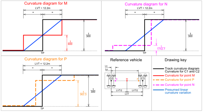
Figure 5. Curvature diagrams
This exercise can be done for other radii and other alignment combinations. The results are similar – the constant curvature will always be found, related to the proportion between the radii of the track alignment. This is true for the range of radii encountered in railway track design. The general form of this curve is a polynomial spline curve, but for radii above 200m and chords (vehicles) of 12-20m the curvature is practically constant, as proven here.
The influence of the bogie was not taken into account but, using the same procedure, it can be proven that each bogie will add another short intermediate constant curvature. For point M, the middle point of the reference chord – assimilated to the vehicle centre of mass – this will bring the curvature variation acceptable close to the presumed linear curvature variation, justifying the definition of the virtual transition. As we move away from the centre of the vehicle the drop in curvature is more significant. For the points located at the bogie area the curvature variation is practically identical with the track curvature, showing the same sudden change in curvature, without any significant intermediate element.
Based on the equations presented here, it can be demonstrated that the gradual acquisition of angular velocity mentioned in the definition of the Virtual Transition Principle really happens. But the angular velocity and its variation is not considered a design constraint by the track design standards and none of the cant and alignment parameters, as they are defined today, are explicitly dependant of it. Nevertheless, its significance is highlighted briefly in the informative Annex A of the European Norm BS EN13803-1(2010).
This exercise demonstrates that the theory behind the Virtual Transition is more complex phenomenon, simplified by the standard to define an easy to understand and use design constraint, similar as concept with the design constraints for a real transition.
References
- BS EN 13803-1 (2010) Railway Applications – Track – Track alignment parameters – Track gauges 1435 and wider – Part 1: Plain Line. British Standards Institution, London.
- BS EN 13803-2 (2006) Railway Applications – Track – Track alignment parameters – Track gauges 1435 and wider – Part 2: Switches and crossings and comparable alignment design situations with abrupt changes of curvature. British Standards Institution, London.
- NR/L2/TRK/2049 (2010) Track Design Handbook, Network Rail.
- NR/L2/TRK/2102 (2010) Design and Construction of Track, Network Rail.
- S1157 (2014) Track – Performance, Design and Construction. London Underground.
- Cope, Geoffrey (1993) British Railway Track – Design, Construction and Maintenance, Permanent Way Institution, Echo Press, Loughborough.
- Radu, Constantin (2003) Rectificarea si retrasarea curbelor de cale ferata (Rectification and realignment of the railway track curves). Track geometry course. Technical University of Civil Engineering Bucharest.
.JPG)

No comments:
Post a Comment